


Causal modeling in large-scale data to improve identification of adults at risk for combined and common variable immunodeficiencies, NPJ Digital Medicine (2025)
This is a short HOWTO describing the code for the paper “Causal Modeling in Large-Scale Data to Improve Identification of Adults at Risk for Combined and Common Variable Immunodeficiencies Infodemiology Data using Dynamic Bayesian Networks” by Papanastasiou, Scutari, Tachdjian, Hernandex-Trujillo, Raasch, Billmeyer, Vasilyev and Ivanov. (2025, NPJ Digital Medicine).
Loading the data
Load the data:
- Encode all variables as factors.
- Rename the target variable toe
PID. - Remove the metadata that are not used in the analysis.
> cohorts = vector(4, mode = "list")
>
> for (c in seq_along(cohorts)) {

+   # read the data file...
+   filename = paste0("COHORT_", c, "_SF_THRESHOLD_5.csv")
+   cohorts[[c]] = read.csv(filename, head = TRUE, colClasses = "factor")
+   # ... rename the target variable...
+   names(cohorts[[c]])[names(cohorts[[c]]) == "cohort_flag"] = "PID"
+   # ... and remove the metadata.
+   cohorts[[c]] = cohorts[[c]][, setdiff(colnames(cohorts[[c]]), c("patient_id", "cohort_type"))]

+ }#FOR
Cleaning and preparing the data
All variables are complete; there are no missing values.
> incomplete = lapply(seq_along(cohorts), function(c) {

+   table(factor(sapply(cohorts[[c]], anyNA), levels = c("FALSE", "TRUE")))

+ })
| FALSE | TRUE | |
|---|---|---|
| Cohort 1 | 563 | 0 |
| Cohort 2 | 560 | 0 |
| Cohort 3 | 395 | 0 |
| Cohort 4 | 329 | 0 |
Some variables are aliases of PI: we remove them to avoid leaking information to the causal network
learning procedure.
> leaks = c(
+   "immunity_deficiency",
+   "other_specified_immunodeficiencies",
+   "nonfamilial_hypogammaglobulinemia",
+   "certain_disorders_involving_the_immune_mechanism",
+   "immunodeficiency_with_predominantly_antibody_defects",
+   "other_immunodeficiencies",
+   "immunodeficiency__unspecified",
+   "selective_deficiency_of_immunoglobulin_g__igg__subclasses",
+   "selective_deficiency_of_immunoglobulin_a__iga_",
+   "selective_deficiency_of_immunoglobulin_m__igm_",
+   "immunodeficiency_with_predominantly_antibody_defects__unsp",
+   "antibody_defic_w_near_norm_immunoglob_or_w_hyperimmunoglob",
+   "other_immunodeficiencies_with_predominantly_antibody_defects",
+   "deficiency_of_humoral_immunity",
+   "other_specified_disorders_involving_the_immune_mechanism"
+ )
>
> for (c in seq_along(cohorts))
+   cohorts[[c]] = cohorts[[c]][, !(colnames(cohorts[[c]]) %in% leaks)]
Checking pairwise associations to identify variables that are (more or less) identical and, therefore, carry the same information. For each possible pair of variables, take the corresponding columns in the data and run a Pearson's χ2 test to check how much they are associated. Each p-value p = 0 means that the two variables in the pair take the same value in each observation in the data. The implication is that they are numerically identical, and one of them is completely redundant in the analysis because it does not provide any information over the other. Each p-value p ≈ 0 means the two variables take the same value in almost all observations. The implication is that keeping both in the analysis is only marginally useful because those variables provide essentially the same information.
> check.similarity = function(data) {

+   pvalues = combn(colnames(data), 2)
+   pvalues = data.frame(var1 = pvalues[1, ], var2 = pvalues[2, ], p = NA_real_)

+   for (i in seq(nrow(pvalues)))
+     pvalues[i, "p"] = ci.test(pvalues[i, "var1"], pvalues[i, "var2"],
+                               data = data, test = "x2")$p.value

+   return(pvalues)

+ }#CHECK.SIMILARITY
>
> pvalues = parLapply(cl, cohorts, check.similarity)
Plotting the p-values from a Pearson's χ2 test, we can see many pairs of variables that are very strongly associated.
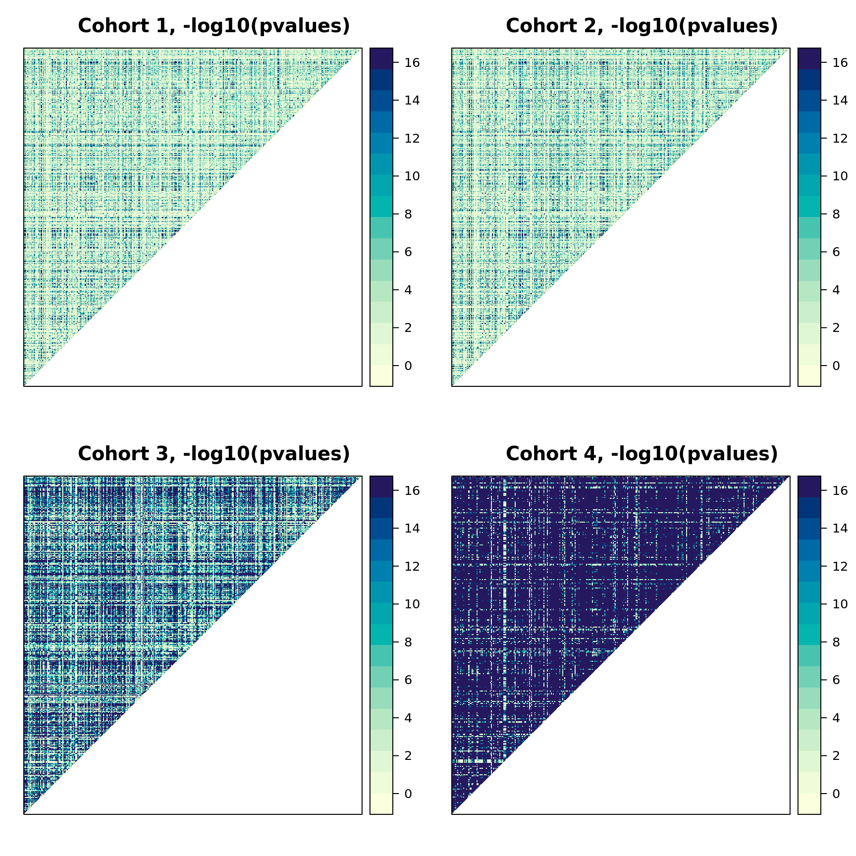
We do not want too many such variables in the data because it is very difficult to separate their causal effects, and causal discovery algorithms can spend significant time trying to do that. Therefore, we first remove duplicate variables (that is, one variable in each pair of variables that take identical values).
> deduplicate = function(data, pvalues, threshold = .Machine$double.eps) {

+   keep = structure(rep(TRUE, ncol(data)), names = colnames(data))

+   if (missing(pvalues))
+     pvalues = flag.redundant(data)

+   # scan the variables...
+   for (var in colnames(data)) {

+     # ... for each variable still under consideration...
+     if (!keep[var])
+       next
+     # ... find the variables that are (nearly) identical to it...
+     to.drop =
+       pvalues[(pvalues$var1 == var) & (pvalues$p < threshold), "var2"]
+     # ... and that are still under consideration...
+     to.drop = intersect(to.drop, names(which(keep)))
+     # .. and drop them.
+     keep[to.drop] = FALSE

+     # never ever drop PID.
+     keep["PID"] = TRUE

+   }#FOR

+   return(keep)

+ }#DEDUPLICATE
We must set a threshold for removing the variables: the values below are a practical compromise between the predictive accuracy of the models we can learn from them and the running time of the learning process (approximately 1 hour per cohort).
> # set the thresholds for inclusion...
> thresholds = c(1e-20, 1e-20, 1e-84, 1e-84)
> # ... process the cohorts...
> clean.cohorts = vector(length(cohorts), mode = "list")
>
> for (c in seq_along(cohorts)) {

+   keep = deduplicate(cohorts[[c]], pvalues = pvalues[[c]],
+                      threshold = thresholds[[c]])

+   clean.cohorts[[c]] = cohorts[[c]][, keep]

+   # ... and add the cohort number as an attribute.
+   attr(clean.cohorts[[c]], "cohort.id") = c

+ }#FOR
Structure learning
We learn the structure of the causal networks using tabu search and BIC inside bootstrap aggregation (bagging).
> inclusion.probabilities = function(data) {

+   bl = data.frame(from = "PID", to = setdiff(colnames(data), "PID"))
+   boot.strength(data, R = 200, algorithm = "tabu",
+     algorithm.args = list(tabu = 50, blacklist = bl), shuffle = TRUE)

+ }#INCLUSION.PROBABILITIES
>
> arc.strengths = parLapply(cl, clean.cohorts, inclusion.probabilities)
The arc strengths represent the probabilities of inclusion of all possible arcs. We threshold them with the data-driven threshold from Scutari & Nagarajan to produce a consensus causal DAG for each cohort.
> consensus.dags = lapply(arc.strengths, averaged.network)
Key summary statistics for each DAG are as follows. Note that all arc directions are uniquely identified from the data.
| Nodes | Arcs | Directed arcs | Undirected arcs | |
|---|---|---|---|---|
| Cohort 1 | 241 | 229 | 229 | 0 |
| Cohort 2 | 245 | 245 | 245 | 0 |
| Cohort 3 | 212 | 457 | 457 | 0 |
| Cohort 4 | 22 | 64 | 64 | 0 |
Mapping variable clusters
Each variable we exclude from the analysis is nearly identical to at least one of the variables we retain. Therefore, it is possible to replace the variables in the DAGs with other variables that are semantically different but numerically almost identical. Here, we map the possible replacements.
> map.clusters = function(full.data, reduced.data, file) {

+   dropped = setdiff(colnames(full.data), colnames(reduced.data))
+   kept = colnames(reduced.data)

+   match = data.frame(
+     `in the DAG` = character(0),
+     `can be replaced with` = character(0)
+   )

+   for (k in setdiff(kept, "PID")) {

+     for (d in dropped) {

+       pvalue = ci.test(k, d, data = full.data, test = "x2")$p.value

+       if (pvalue < .Machine$double.eps)
+         match[nrow(match) + 1, ] = c(k, d)

+     }#FOR

+   }#FOR

+   write.csv(match, file = file, row.names = FALSE)

+ }#MAP.CLUSTERS
>
> clusterExport(cl, list("map.clusters"))
> parSapply(cl, seq_along(cohorts), function(c, cohorts, clean.cohorts) {

+   map.clusters(full.data = cohorts[[c]], reduced.data = clean.cohorts[[c]],
+                file = paste0("clusters.cohort.", c, ".csv"))

+ }, cohorts = cohorts, clean.cohorts = clean.cohorts)
Based on clinical prior knowledge, we use these clusters to replace some of the previously selected variables with equivalent ones that are more appropriate in context.
> substitutions = list(
+   matrix(c(
+     "accident", "complications_after_procedure",
+     "sexually_transmitted_infections__not_hiv_or_hepatitis_", "other_disorders_of_lipoid_metabolism",
+     "bone_marrow_or_stem_cell_transplant", "disorders_involving_the_immune_mechanism",
+     "cancer_of_other_lymphoid__histiocytic_tissue", "non_hodgkins_lymphoma",
+     "decreased_white_blood_cell_count", "pancytopenia",
+     "symptoms_concerning_nutrition__metabolism__and_development", "failure_to_thrive_and_developmental_disorders",
+     "anorexia", "nausea_and_vomiting",
+     "effects_of_other_external_causes", "viral_infection",
+     "fracture_of_vertebral_column_without_mention_of_spinal_cord_injury", "musculoskeletal disorders",
+     "opiates_and_related_narcotics_causing_adverse_effects_in_therapeutic_use", "encounter_for_long_term__current__use_of_medications",
+     "acidosis", "septic_shock",
+     "care_provider_dependency", "acute_renal_failure",
+     "sexually_transmitted_infections__not_hiv_or_hepatitis_", "contusion",
+     "superficial_injury_without_mention_of_infection", "injury__nos",
+     "wound_dressing", "open_wounds_of_extremities",
+     "encounter_for_contraceptive_and_procreative_management", "hypothyroidism_nos"),
+   byrow = TRUE, ncol = 2, dimnames = list(NULL, c("original", "replacement"))),
+   matrix(c(
+     "bone_marrow_or_stem_cell_transplant", "disorders_involving_the_immune_mechanism",
+     "complications_of_transplants_and_reattached_limbs", "bacteremia",
+     "complication_due_to_other_implant_and_internal_device", "complications_of_surgical_and_medical_procedures",
+     "deep_vein_thrombosis__dvt_", "anemia_of_chronic_disease",
+     "supplementary_factors_related_to_causes_of_morbidity_classified_elsewhere", "personal_history_of_allergy_to_medicinal_agents",
+     "foreign_body_injury", "dysphagia",
+     "pseudomonal_pneumonia", "bronchiectasis",
+     "other_symptoms", "diarrhea",
+     "fever_of_unknown_origin", "influenza",
+     "atopic_contact_dermatitis_due_to_other_or_unspecified", "disorder_of_skin_and_subcutaneous_tissue_nos",
+     "pruritus_and_related_conditions", "allergies__other",
+     "abdominal_pain", "viral_infection",
+     "anemia_in_neoplastic_disease", "non_hodgkins_lymphoma",
+     "allergic_rhinitis", "asthma",
+     "pneumonitis_due_to_inhalation_of_food_or_vomitus", "pneumococcal_pneumonia",
+     "symptoms_involving_respiratory_system_and_other_chest_symptoms", "lymphadenitis",
+     "other_pulmonary_inflamation_or_edema", "acute_renal_failure"),
+   byrow = TRUE, ncol = 2, dimnames = list(NULL, c("original", "replacement"))),
+   matrix(c(
+     "antineoplastic_and_immunosuppressive_drugs_causing_adverse_effects", "pancytopenia",
+     "anorexia", "encounter_for_long_term__current__use_of_medications",
+     "blood_vessel_replaced", "neutropenia",
+     "bone_marrow_or_stem_cell_transplant", "failure_to_thrive",
+     "short_stature",    "symptoms_concerning_nutrition__metabolism__and_development",
+     "lack_of_coordination", "encephalopathy__not_elsewhere_classified",
+     "other_disorders_of_soft_tissues", "gastritis_and_duodenitis",
+     "symptoms_involving_cardiovascular_system", "asthma",
+     "visual_disturbances", "anxiety_disorder",
+     "acidosis", "bacteremia",
+     "hormones_and_synthetic_substitutes_causing_adverse_effects_in_therapeutic_use", "edema",
+     "other_abnormal_blood_chemistry", "autoimmune_disease_nec",
+     "complications_of_surgical_and_medical_procedures", "abnormal_findings_examination_of_lungs",
+     "complications_of_transplants_and_reattached_limbs", "pleurisy__pleural_effusion",
+     "complication_due_to_other_implant_and_internal_device", "respiratory_failure",
+     "supplementary_factors_related_to_causes_of_morbidity_classified_elsewhere", "asphyxia_and_hypoxemia",
+     "chronic_kidney_disease__stage_iii", "chronic_kidney_disease"),
+   byrow = TRUE, ncol = 2, dimnames = list(NULL, c("original", "replacement"))),
+   matrix(c(
+     "diseases_of_white_blood_cells", "autoimmune_disease_nec",
+     "abdominal_pain", "viral_infection",
+     "oth_contact_w_and__suspected__exposures_hazardous_to_health", "disorders_involving_the_immune_mechanism",
+     "septal_deviations_turbinate_hypertrophy", "asthma",
+     "convulsions", "chronic_sinusitis",
+     "atrial_fibrillation", "bacterial_pneumonia",
+     "epistaxis_or_throat_hemorrhage", "bronchitis",
+     "conjunctivitis__infectious", "allergic_rhinitis",
+     "allergic_reaction_to_food", "develomental_delays_and_disorders",
+     "neoplasm_of_uncertain_behavior", "non_hodgkins_lymphoma",
+     "impacted_cerumen", "chronic_pharyngitis_and_nasopharyngitis",
+     "foreign_body_injury", "asphyxia_and_hypoxemia",
+     "abnormal_heart_sounds", "abnormal_electrocardiogram__ecg___ekg_",
+     "kyphoscoliosis_and_scoliosis", "noninfectious_gastroenteritis",
+     "attention_deficit_hyperactivity_disorder", "chronic_kidney_disease",
+     "fracture_of_unspecified_bones", "gastritis_and_duodenitis__nos",
+     "normal_bmi", "bacteremia",
+     "encounter_for_contraceptive_and_procreative_management", "hypothyroidism_nos"),
+   byrow = TRUE, ncol = 2, dimnames = list(NULL, c("original", "replacement")))
+ )
>
> for (d in seq_along(consensus.dags)) {

+   labels = nodes(consensus.dags[[d]])
+   for (i in seq(nrow(substitutions[[d]])))
+     labels[labels == substitutions[[d]][i, "original"]] = substitutions[[d]][i, "replacement"]
+   nodes(consensus.dags[[d]]) = labels

+ }#FOR
Below are the full causal networks for the cohorts, with the updated node sets.

And here are the respective subnetworks around PID, spanning all the nodes within a distance of
three arcs.

Parameter learning
We estimate the parameters of the consensus networks by maximum likelihood. The sample size is large enough that using regularised posterior parameter estimates does not increase the accuracy of the models.
> estimate.parameters = function(dag, data) {

+   bn.fit(cextend(dag), data, method = "mle", replace.unidentifiable = TRUE)

+ }#ESTIMATE.PARAMETERS
>
> consensus.fitted = lapply(seq_along(consensus.dags), function(d) {

+   estimate.parameters(consensus.dags[[d]], data = clean.cohorts[[d]])

+ })
All the parameters are identifiable from the data: the conditional probability tables associated with the nodes
contain no NAs.
| Any unidentifiable | |
|---|---|
| Cohort 1 | FALSE |
| Cohort 2 | FALSE |
| Cohort 3 | FALSE |
| Cohort 4 | FALSE |
Almost no parameters are too close to 0 and 1, so we do not expect numerical problems
when computing conditional probabilities during inference.
| FALSE | TRUE | |
|---|---|---|
| Cohort 1 | 237 | 4 |
| Cohort 2 | 242 | 3 |
| Cohort 3 | 196 | 16 |
| Cohort 4 | 18 | 4 |
The number of parameters of the networks learned from the cohorts is as follows.
| Number of parameters | |
|---|---|
| Cohort 1 | 548 |
| Cohort 2 | 562 |
| Cohort 3 | 1171 |
| Cohort 4 | 219 |
Inference
Predictive accuracy
We measure the predictive accuracy using the standard set of measures for classifiers: sensitivity, specificity, accuracy and the area under the ROC curve.
> accuracy.metrics = function(obs, pred, probs, cohort.id) {

+   # tally up the relevant counts.
+   counts = table(obs = obs, pred = pred)
+   TP = counts["1", "1"]
+   TN = counts["0", "0"]
+   FP = counts["0", "1"]
+   FN = counts["1", "0"]

+   # classification error.
+   clerr = (FN + FP) / sum(counts)

+   # sensitivity, specificity and accuracy.
+   sens = TP / (TP + FP)
+   spec = TN / (TN + FN)
+   acc = (TP + TN) / sum(counts)

+   # area under the ROC curve.
+   roc = ROCR::prediction(probs, obs)
+   auroc = ROCR::performance(roc, measure = "auc")@y.values[[1]]

+   if (!missing(cohort.id)) {

+     # produce the ROC curve...
+     roc.curve = ROCR::performance(roc, measure = "tpr", x.measure = "fpr")
+     # ... and save the object with the curve points.
+     saveRDS(roc.curve, file = paste0("roc.points.", cohort.id, ".rds"))

+   }#THEN

+   return(c(clerr = clerr, sens = sens, spec = spec, acc = acc, auroc = auroc))

+ }#ACCURACY.METRICS
We estimate them using the gold-standard 10 runs of 10-fold cross-validation and the same structure learning approach we used to learn the consensus networks.
> crossvalidate.single.network = function(data, runs = 10) {

+   learn.single.dag = function(data) {

+     bl = data.frame(from = "PID", to = setdiff(colnames(data), "PID"))
+     tabu(data, blacklist = bl, score = "bic", tabu = 50)

+   }#LEARN.SINGLE.DAG

+   output = vector(runs, mode = "list")

+   # for the required number of replicates...
+   for (r in seq(runs)) {

+     all = data.frame(
+       probs = numeric(nrow(data)),
+       obs = factor(numeric(nrow(data)), levels = c("0", "1")),
+       preds = factor(numeric(nrow(data)), levels = c("0", "1"))
+     )

+     # ... shuffle and split the observations into 10 folds...
+     pick = suppressWarnings(split(sample(seq(nrow(data))), 1:10))
+     # ... and for each fold...
+     for (j in seq_along(pick)) {

+       # ... use it as the test set, merging the rest into the training set...
+       test.set = data[pick[[j]], ]
+       training.set = data[-pick[[j]], ]
+       # ... learn the structure and the parameters...
+       dag = learn.single.dag(training.set)
+       bn = estimate.parameters(dag, training.set)
+       # ... get the predicted PID values, observed PID values, and
+       # prediction probabilities...
+       pred = predict(bn, data = test.set, node = "PID", method = "parents",
+                      prob = TRUE)
+       all[pick[[j]], "obs"] = test.set[, "PID"]
+       all[pick[[j]], "probs"] = attr(pred, "prob")["1", ]
+       all[pick[[j]], "preds"] = pred

+     }#FOR

+     # compute the performance measures (concatenating the cohort and run numbers
+     # to save all the outputs).
+     output[[r]] = accuracy.metrics(obs = all[, "obs"], pred = all[, "preds"],
+                     probs = all[, "probs"],
+                     cohort.id = paste0(attr(data, "cohort.id"), ".", r))

+   }#FOR

+   return(do.call(rbind, output))

+ }#CROSSVALIDATE.SINGLE.NETWORK
>
> metrics = parLapply(cl, clean.cohorts, crossvalidate.single.network)
| Average | Standard deviation | |
|---|---|---|
| Classification error | 0.25 | 0.00 |
| Sensitivity | 0.84 | 0.00 |
| Specificity | 0.69 | 0.00 |
| Accuracy | 0.75 | 0.00 |
| Area under the ROC curve | 0.77 | 0.01 |
| Average | Standard deviation | |
|---|---|---|
| Classification error | 0.28 | 0.00 |
| Sensitivity | 0.70 | 0.00 |
| Specificity | 0.75 | 0.00 |
| Accuracy | 0.72 | 0.00 |
| Area under the ROC curve | 0.75 | 0.00 |
| Average | Standard deviation | |
|---|---|---|
| Classification error | 0.35 | 0.00 |
| Sensitivity | 0.88 | 0.00 |
| Specificity | 0.59 | 0.00 |
| Accuracy | 0.65 | 0.00 |
| Area under the ROC curve | 0.63 | 0.00 |
| Average | Standard deviation | |
|---|---|---|
| Classification error | 0.41 | 0.00 |
| Sensitivity | 0.78 | 0.00 |
| Specificity | 0.55 | 0.00 |
| Accuracy | 0.59 | 0.00 |
| Area under the ROC curve | 0.61 | 0.00 |
Here are the corresponding ROC curves, with the average ROC curve overlaid.

Interventions and odds ratios
We use interventions to compute the odds of a PID diagnosis when each of the other conditions is diagnosed (or not). We compute them using approximate inference because exact inference requires more than 16GB of memory for the causal network learned from cohort 3.
> condition.odds = function(fitted) {

+   odds = data.frame(
+     with = numeric(nnodes(fitted) - 1),
+     without = numeric(nnodes(fitted) - 1),
+     row.names = setdiff(nodes(fitted), "PID")
+   )

+   for (node in row.names(odds)) {

+     # perform the intervention to introduce the condition (or not)...
+     with.condition = as.list(structure("1", names = node))
+     fitted.with.condition = mutilated(fitted, evidence = with.condition)
+     # perform the intervention to remove the condition...
+     without.condition = as.list(structure("0", names = node))
+     fitted.without.condition = mutilated(fitted, evidence = without.condition)

+     # ... and compute the odds of PID.
+     particles = cpdist(fitted.with.condition, nodes = c("PID", node),
+                        evidence = TRUE, n = 10^5)
+     probs = prop.table(table(particles))
+     odds.with.condition = probs["1", "1"] / probs["0", "1"]

+     particles = cpdist(fitted.without.condition, nodes = c("PID", node),
+                        evidence = TRUE, n = 10^5)
+     probs = prop.table(table(particles))
+     odds.without.condition = probs["1", "0"] / probs["0", "0"]

+     # save both odds.
+     odds[node, ] = c(odds.with.condition, odds.without.condition)

+   }#FOR

+   return(odds)

+ }#CONDITION.ODDS
>
> pid.odds = parLapply(cl, consensus.fitted, condition.odds)

Predicting Across Cohorts
In addition to measuring the accuracy of the causal networks for the cohorts they have been learned from, it is interesting to measure how well they generalise to other cohorts.
> accuracy.metrics.wrapper = function(model, data) {

+   # gather observed PID values, predicted PID values and their probabilities.
+   obs = data[, "PID"]
+   pred = predict(model, node = "PID", data = data, method = "bayes-lw",
+                  n = 1000, prob = TRUE)
+   probs = attr(pred, "prob")["1", ]
+   obs = obs[!is.na(pred)]
+   probs = probs[!is.na(pred)]
+   pred = pred[!is.na(pred)]

+   accuracy.metrics(obs, pred, probs)

+ }#ACCURACY.METRICS.WRAPPER
>
> metrics = data.frame(
+   expand.grid("From cohort" = 1:4, "To cohort" = 1:4),
+   "Classification error" = NA_real_,
+   "Sensitivity" = NA_real_,
+   "Specificity" = NA_real_,
+   "Accuracy" = NA_real_,
+   "Area under the ROC curve" = NA_real_,
+   check.names = FALSE
+ )
>
> for (f in seq_along(consensus.fitted)) {

+   for (c in setdiff(seq_along(cohorts), f)) {

+     metrics[metrics[, "From cohort"] == f & metrics[, "To cohort"] == c, -(1:2)] =
+       accuracy.metrics.wrapper(consensus.fitted[[f]], cohorts[[c]])

+   }#FOR

+ }#FOR
| From cohort | To cohort | Classification error | Sensitivity | Specificity | Accuracy | Area under the ROC curve |
|---|---|---|---|---|---|---|
| 1 | 2 | 0.259 | 0.831 | 0.690 | 0.741 | 0.766 |
| 1 | 3 | 0.401 | 0.764 | 0.562 | 0.599 | 0.632 |
| 1 | 4 | 0.427 | 0.756 | 0.543 | 0.573 | 0.605 |
| 2 | 1 | 0.372 | 0.600 | 0.678 | 0.628 | 0.703 |
| 2 | 3 | 0.402 | 0.636 | 0.578 | 0.598 | 0.611 |
| 2 | 4 | 0.427 | 0.620 | 0.553 | 0.573 | 0.580 |
| 3 | 1 | 0.301 | 0.884 | 0.634 | 0.699 | 0.698 |
| 3 | 2 | 0.305 | 0.870 | 0.633 | 0.695 | 0.719 |
| 3 | 4 | 0.429 | 0.811 | 0.541 | 0.571 | 0.593 |
| 4 | 1 | 0.335 | 0.796 | 0.614 | 0.665 | 0.689 |
| 4 | 2 | 0.338 | 0.787 | 0.613 | 0.662 | 0.688 |
| 4 | 3 | 0.412 | 0.787 | 0.555 | 0.588 | 0.608 |
Focusing on the area under the ROC curve.

Predicting the controls from the same cohort
From causal effect point of view, it is also interesting to predict only the controls.
> accuracy.controls.wrapper = function(model, target.cohort) {

+   target.cohort = subset(target.cohort, PID == "0")
+   target.cohort$PID = relevel(target.cohort$PID, ref = "1")
+   levels(target.cohort$PID) = c("0", "1")
+   obs = target.cohort[, "PID"]
+   pred = predict(model, node = "PID", data = target.cohort,
+            method = "bayes-lw", n = 1000, prob = TRUE)
+   probs = attr(pred, "prob")["1", ]
+   obs = obs[!is.na(pred)]
+   probs = probs[!is.na(pred)]
+   pred = pred[!is.na(pred)]

+   pairs = data.frame(obs = obs, pred = pred, probs = probs)
+   # ROCR refuses to work without at least one true positive, add a dummy one.
+   pairs = rbind(pairs, c(0, 0, 1))

+   accuracy.metrics(pairs$obs, pairs$pred, pairs$probs)

+ }#ACCURACY.POOLED.WRAPPER
>
> metrics = data.frame(
+   "From cohort" = 1:4,
+   "Classification error" = NA_real_,
+   "Sensitivity" = NA_real_,
+   "Specificity" = NA_real_,
+   "Accuracy" = NA_real_,
+   "Area under the ROC curve" = NA_real_,
+   check.names = FALSE
+ )
>
> for (f in seq_along(consensus.fitted)) {

+  metrics[metrics[, "From cohort"] == f, -1] =
+     accuracy.controls.wrapper(consensus.fitted[[f]], cohorts[[f]])

+ }#FOR
| From cohort | Sensitivity | Specificity | Accuracy |
|---|---|---|---|
| 1 | 0.001 | 0.001 | 0.001 |
| 2 | 0.002 | 0.002 | 0.002 |
| 3 | 0.000 | 0.000 | 0.000 |
| 4 | 0.000 | 0.000 | 0.000 |
Sensitivity to the Model Averaging Threshold
The threshold used to include arcs in the consensus networks is estimated directly from the data as 0.5 for all four cohorts. Increasing or decreasing it by 0.05 (a 10% change in either direction) allows us to assess the sensitivity of the consensus networks to its value.
> clusterExport(cl, c("estimate.parameters", "accuracy.metrics", "accuracy.metrics.wrapper"))

> sensitivity = parLapply(cl, seq_along(cohorts),
+     function(cohorts, strengths, c) {
+       # estimate the default threshold...
+       thresold = inclusion.threshold(strengths[[c]])
+       # ... create the consensus DAG by increasing/decreasing it...
+       baseline = averaged.network(strengths[[c]], threshold = thresold)
+       sparse = averaged.network(strengths[[c]], threshold = thresold + 0.05)
+       dense = averaged.network(strengths[[c]], threshold = thresold - 0.05)
+       # ... fit the parameters of the consensus networks...
+       baseline = estimate.parameters(baseline, cohorts[[c]][, nodes(baseline)])
+       sparse = estimate.parameters(sparse, cohorts[[c]][, nodes(sparse)])
+       dense = estimate.parameters(dense, cohorts[[c]][, nodes(dense)])
+       # ... and compute the metrics for all of them.
+       metrics = list()

+       for (val in setdiff(seq_along(cohorts), c)) {

+         baseline.metrics = accuracy.metrics.wrapper(baseline, cohorts[[val]])
+         new.metrics = list(
+           c("From cohort" = c, "To cohort" = val, "Threshold" = "sparse",
+               accuracy.metrics.wrapper(sparse, cohorts[[val]]) - baseline.metrics),
+           c("From cohort" = c, "To cohort" = val, "Threshold" = "dense",
+               accuracy.metrics.wrapper(dense, cohorts[[val]]) - baseline.metrics)
+         )

+         # add the proportion of PID parents shared with the original network.
+         new.metrics[[1]]$effects =
+           length(intersect(parents(sparse, "PID"), parents(baseline, "PID"))) /
+             length(parents(baseline, "PID"))
+         new.metrics[[2]]$effects =
+           length(intersect(parents(dense, "PID"), parents(baseline, "PID"))) /
+             length(parents(baseline, "PID"))

+         metrics = c(metrics, new.metrics)

+       }#FOR

+       return(metrics)

+   }, cohorts = cohorts, strengths = arc.strengths)
The table below reports the difference in accuracy metrics for the resulting sparser (threshold + 0.05) and denser (threshold - 0.05) consensus networks compared to those of the original consensus network (unchanged threshold). In addition, the last column reports how many parents of PID from the original consensus network are present in the sparser and denser networks from the same cohort.
| From cohort | To cohort | Threshold | Classification error | Sensitivity | Specificity | Accuracy | Area under the ROC curve | Shared Direct Causal Effects |
|---|---|---|---|---|---|---|---|---|
| 1 | 2 | sparse | 0.0000 | 0.0000 | 0.0000 | 0.0000 | -0.0156 | 0.75 |
| 1 | 2 | dense | 0.0007 | 0.0015 | -0.0022 | -0.0007 | 0.0063 | 1.00 |
| 1 | 3 | sparse | 0.0000 | -0.0006 | 0.0000 | 0.0000 | -0.0276 | 0.75 |
| 1 | 3 | dense | -0.0004 | 0.0012 | 0.0003 | 0.0004 | -0.0101 | 1.00 |
| 1 | 4 | sparse | 0.0001 | -0.0008 | 0.0000 | -0.0001 | -0.0307 | 0.75 |
| 1 | 4 | dense | 0.0001 | -0.0004 | -0.0001 | -0.0001 | 0.0023 | 1.00 |
| 2 | 1 | sparse | 0.0006 | -0.0006 | -0.0006 | -0.0006 | 0.0049 | 1.00 |
| 2 | 1 | dense | 0.0006 | -0.0006 | -0.0006 | -0.0006 | -0.0009 | 1.00 |
| 2 | 3 | sparse | -0.0007 | 0.0006 | 0.0006 | 0.0007 | -0.0099 | 1.00 |
| 2 | 3 | dense | -0.0011 | 0.0013 | 0.0009 | 0.0011 | -0.0093 | 1.00 |
| 2 | 4 | sparse | 0.0000 | -0.0004 | 0.0000 | 0.0000 | -0.0012 | 1.00 |
| 2 | 4 | dense | 0.0005 | -0.0006 | -0.0004 | -0.0005 | 0.0011 | 1.00 |
| 3 | 1 | sparse | 0.0000 | 0.0000 | 0.0000 | 0.0000 | -0.0106 | 1.00 |
| 3 | 1 | dense | 0.0008 | 0.0000 | -0.0012 | -0.0008 | -0.0094 | 1.00 |
| 3 | 2 | sparse | 0.0000 | 0.0000 | 0.0000 | 0.0000 | -0.0133 | 1.00 |
| 3 | 2 | dense | 0.0002 | 0.0000 | -0.0003 | -0.0002 | -0.0014 | 1.00 |
| 3 | 4 | sparse | 0.0005 | -0.0012 | -0.0003 | -0.0005 | -0.0062 | 1.00 |
| 3 | 4 | dense | -0.0001 | 0.0013 | 0.0000 | 0.0001 | -0.0047 | 1.00 |
| 4 | 1 | sparse | 0.0025 | -0.0058 | -0.0015 | -0.0025 | -0.0042 | 1.00 |
| 4 | 1 | dense | 0.0034 | -0.0089 | -0.0020 | -0.0034 | -0.0005 | 1.00 |
| 4 | 2 | sparse | -0.0013 | 0.0087 | -0.0001 | 0.0013 | 0.0135 | 1.00 |
| 4 | 2 | dense | -0.0032 | 0.0089 | 0.0017 | 0.0032 | 0.0146 | 1.00 |
| 4 | 3 | sparse | -0.0011 | 0.0042 | 0.0006 | 0.0011 | -0.0004 | 1.00 |
| 4 | 3 | dense | -0.0027 | 0.0067 | 0.0015 | 0.0027 | 0.0013 | 1.00 |
Sat May 10 06:16:09 2025 with bnlearn
4.9.3
and R version 4.3.2 (2023-10-31).

