


bnlearn: Practical Bayesian Networks in R
This tutorial aims to introduce the basics of Bayesian network learning and inference using bnlearn and real-world data to explore a typical data analysis workflow for graphical modelling. Key points will include:
- preprocessing the data;
- learning the structure and the parameters of a Bayesian network;
- using the network as a predictive model;
- using the network for inference;
- validating the network by contrasting it with external information.
A Quick introduction
Bayesian networks
Definitions
Bayesian networks (BNs) are defined by:
- a network structure, a directed acyclic graph
 , in which
each node
, in which
each node  corresponds to a random variable
 ;
; - a global probability distribution
 (with parameters
 ),
which can be factorised into smaller local probability distributions according to
the arcs present in the graph.
),
which can be factorised into smaller local probability distributions according to
the arcs present in the graph.
The main role of the network structure is to express the conditional independence relationships among the variables in the model through graphical separation, thus specifying the factorisation of the global distribution:

Each local distribution has its own parameter set  ; and
⋃ is much smaller than
because many parameters are fixed by the fact that the variables they belong
to are independent.
; and
⋃ is much smaller than
because many parameters are fixed by the fact that the variables they belong
to are independent.
So the first component is a directed acyclic graph like this:

And the implication is that:

The second component of a BN is the probability distribution  . The
choice should be such that the BN:
. The
choice should be such that the BN:
- can be learned efficiently from data;
- is flexible (it can encode a reasonable variety of phenomena);
- is easy to query to perform inference.
The three most common choices in the literature (by far), are:
- discrete BNs, in which and the
 ; and
the are the conditional probabilities
; and
the are the conditional probabilities

- Gaussian BNs (GBNs), in which is multivariate normal and the
are univariate normals defined by the linear
regression model

- Conditional linear Gaussian BNs (CLGBNs), in which is a mixture of
multivariate normals and the are either multinomial,
univariate normal or mixtures of normals.
- Discrete are only allowed to have discrete parents (denoted
 ), are assumed to follow a multinomial distribution parameterised
with conditional probability tables;
), are assumed to follow a multinomial distribution parameterised
with conditional probability tables; - continuous are allowed to have both discrete and
continuous parents (denoted
 ,
∪
=
,
∪
=  , and their local distributions are

which can be written as a mixture of linear regressions

against the continuous parents with one component for each configuration of the discrete parents. If
has no discrete parents, the mixture reverts to a single
linear regression.
of the discrete parents. If
has no discrete parents, the mixture reverts to a single
linear regression.
- Discrete
Learning
Model selection and estimation of BNs are collectively known as learning, and are usually performed as a two-step process:
- structure learning, learning the network structure from the data;
- parameter learning, learning the local distributions implied by the structure learned in the previous step.
This workflow is Bayesian; given a data set  and if we denote the
parameters of the global distribution as with
, we have
and if we denote the
parameters of the global distribution as with
, we have

and structure learning is done in practice as

Combined with the fact that the local distribution  decomposes into local distributions that depend only on and its
parents
decomposes into local distributions that depend only on and its
parents

Once we have an estimate for from structure learning, we can
identify the local distributions since we know the parents
of each node; and we can estimate their parameter set
independently from each other. Assuming is sparse, each
involves only few variables and thus estimating its
parameters is computationally simple.
Inference
Inference on BNs usually consists of conditional probability (CP) or maximum a posteriori (MAP) queries. The general idea of a CP query is:
- we have some evidence, that is, we know the values of some variables and we fix the nodes accordingly; and
- we want to look into the probability of some event involving (a subset of) the other variables conditional on the evidence we have.
Say we start from a discrete BN with the DAG used above.

Graphically a CP query looks like this:

On the other hand, the goal of a MAP query is to find the combination of values for (a subset of) the variables in the network that has the highest probability given some evidence. If the evidence is a partially-observed new individual, then performing a MAP query amounts to a classic prediction exercise.

This is more computationally challenging than it sounds because, as a task, it does not decompose along local distributions.
The bnlearn package
bnlearn is designed to provide a flexible simulation suite for methodological research and effective and scalable data analysis tools for working with BNs on real-world data. This is achieved by a modular architecture in which algorithms are decoupled from model assumptions, to make it possible to mix and match the methods found in the literature.

bnlearn leverages the modularity of BNs to achieve this goal:
- learning the structure of the network, or creating one manually, gives an object of
class
bnthat encodes; - learning the parameters for a given structure starts from a
bnobject and gives an object of classbn.fitthat encodes (,
); - inference takes an object of class
bn.fit.
Objects of class bn can be created:
- using a model string encoding each node and its parents;
> dag = model2network("[A][S][E|A:S][O|E][R|E][T|O:R]")
- using the arc set;
> arc.set = matrix(c("A", "E",
+                    "S", "E",
+                    "E", "O",
+                    "E", "R",
+                    "O", "T",
+                    "R", "T"),
+             byrow = TRUE, ncol = 2,
+             dimnames = list(NULL, c("from", "to")))
> dag = empty.graph(c("A", "S", "E", "O", "R", "T"))
> arcs(dag) = arc.set
- or by learning them from data.
> dag = hc(data)
The anatomy of a bn object (documented in ?"bn class") is as follows:
it comprises some metadata on how then bn object was created ($learning);
some relevant graph-theoretic quantities ($nodes, cached for speed); and the arc
set ($arcs).
List of 3
 $ learning:List of 6
  ..$ whitelist: NULL
  ..$ blacklist: NULL
  ..$ test     : chr "none"
  ..$ ntests   : num 0
  ..$ algo     : chr "empty"
  ..$ args     : list()
 $ nodes   :List of 6
  ..$ A:List of 4
  .. ..$ mb      : chr [1:2] "S" "E"
  .. ..$ nbr     : chr "E"
  .. ..$ parents : chr(0)
  .. ..$ children: chr "E"
  ..$ S:List of 4
  .. ..$ mb      : chr [1:2] "A" "E"
  .. ..$ nbr     : chr "E"
  .. ..$ parents : chr(0)
  .. ..$ children: chr "E"
  ..$ E:List of 4
  .. ..$ mb      : chr [1:4] "A" "S" "O" "R"
  .. ..$ nbr     : chr [1:4] "A" "S" "O" "R"
  .. ..$ parents : chr [1:2] "A" "S"
  .. ..$ children: chr [1:2] "O" "R"
  ..$ O:List of 4
  .. ..$ mb      : chr [1:3] "E" "R" "T"
  .. ..$ nbr     : chr [1:2] "E" "T"
  .. ..$ parents : chr "E"
  .. ..$ children: chr "T"
  ..$ R:List of 4
  .. ..$ mb      : chr [1:3] "E" "O" "T"
  .. ..$ nbr     : chr [1:2] "E" "T"
  .. ..$ parents : chr "E"
  .. ..$ children: chr "T"
  ..$ T:List of 4
  .. ..$ mb      : chr [1:2] "O" "R"
  .. ..$ nbr     : chr [1:2] "O" "R"
  .. ..$ parents : chr [1:2] "O" "R"
  .. ..$ children: chr(0)
 $ arcs    : chr [1:6, 1:2] "A" "S" "E" "E" ...
  ..- attr(*, "dimnames")=List of 2
  .. ..$ : NULL
  .. ..$ : chr [1:2] "from" "to"
 - attr(*, "class")= chr "bn"
In contrast, a bn.fit object (documented in ?"bn.fit class") is simply
a named list with one element for each node, comprising its parameters (prob for
discrete nodes, coef and sd for Gaussian nodes) and the labels of its
parents and children.
> survey$R
  Parameters of node R (multinomial distribution)

Conditional probability table:

       E
R       high  uni
  small 0.25 0.20
  big   0.75 0.80
> str(survey$R)
List of 4
 $ node    : chr "R"
 $ parents : chr "E"
 $ children: chr "T"
 $ prob    : table [1:2, 1:2] 0.25 0.75 0.2 0.8
  ..- attr(*, "dimnames")=List of 2
  .. ..$ R: chr [1:2] "small" "big"
  .. ..$ E: chr [1:2] "high" "uni"
 - attr(*, "class")= chr "bn.fit.dnode"
Objects of class bn.fit can be created:
- by learning the parameters from data using
bn.fit();> fitted = bn.fit(dag, data = survey.data)
- by providing the parameters to
custom.fit().> A.lv = c("young", "adult", "old") > S.lv = c("M", "F") > E.lv = c("high", "uni") > O.lv = c("emp", "self") > R.lv = c("small", "big") > T.lv = c("car", "train", "other") > A.prob = array(c(0.30, 0.50, 0.20), dim = 3, dimnames = list(A = A.lv)) > S.prob = array(c(0.60, 0.40), dim = 2, dimnames = list(S = S.lv)) > O.prob = array(c(0.96, 0.04, 0.92, 0.08), dim = c(2, 2), + dimnames = list(O = O.lv, E = E.lv)) > R.prob = array(c(0.25, 0.75, 0.20, 0.80), dim = c(2, 2), + dimnames = list(R = R.lv, E = E.lv)) > E.prob = array(c(0.75, 0.25, 0.72, 0.28, 0.88, 0.12, 0.64, + 0.36, 0.70, 0.30, 0.90, 0.10), dim = c(2, 3, 2), + dimnames = list(E = E.lv, A = A.lv, S = S.lv)) > > T.prob = array(c(0.48, 0.42, 0.10, 0.56, 0.36, 0.08, 0.58, + 0.24, 0.18, 0.70, 0.21, 0.09), dim = c(3, 2, 2), + dimnames = list(T = T.lv, O = O.lv, R = R.lv)) > cpt = list(A = A.prob, S = S.prob, E = E.prob, O = O.prob, R = R.prob, T = T.prob) > survey = custom.fit(dag, cpt)
Finally, starting from a bn.fit object we can:
- generate random samples;
> rbn(survey, n = 10)
A E O R S T 1 old uni emp big M car 2 old high emp small F car 3 adult uni emp big F car 4 old uni self big M train 5 young high emp big M car 6 young high emp small F train 7 young high emp big F train 8 adult uni emp big M car 9 young high self small M car 10 young uni emp big M car - predict new observations;
> newdata = data.frame(A = factor("young", levels = A.lv),
+                      S = factor("F", levels = S.lv),
+                      E = factor("uni", levels = E.lv),
+                      O = factor("self", levels = O.lv),
+                      R = factor("big", levels = R.lv))
> predict(survey, node = "T", data = newdata)
[1] car
Levels: car train other
- compute probabilities with CP queries;
> cpquery(survey, event = (S == "M") & (T == "car"), evidence = (E == "high"))
[1] 0.3479195
- generate (weighted) observations from arbitrary conditional distributions.
> SxT = cpdist(survey, nodes = c("S", "T"), evidence = (E == "high"))
> head(SxT)
  S     T
1 M train
2 M other
3 M   car
4 M   car
5 F other
6 F   car
> table(SxT)
   T
S    car train other
  M 1248   659   352
  F  821   433   218
A Bayesian network analysis of malocclusion data
Bayesian Networks Analysis of Malocclusion Data.
[ arXiv (preprint) |
html |
pdf |
online supplementary material ]
M. Scutari, P. Auconi, G. Caldarelli and L. Franchi (2017).
Scientific Reports, 7(15326).
The problem: Patients affected by Class III malocclusion (characterised by the protrusion of lower dental arch) suffer from a skeletal imbalance that is established early in life, and that becomes more pronounced during puberty and until skeletal maturation is complete. Predicting treatment success or failure early in a single Class III patient makes it easier to correct it, but it is difficult to do just from a small number of morphometric determinants is problematic. The reason for that is that Class III malocclusion is rarely a consequence of an abnormality in a single craniofacial component, so individual clinical and radiological measurements are likely to be less indicative than the interplay between the measurements themselves.
The task:
- We learn a BN and use it to determine and visualise the interactions among various Class III malocclusion maxillofacial features during growth and treatment.
- We test its consistency by verifying some commonly accepted hypotheses on the evolution of these skeletal imbalances.
- We show that untreated subjects develop different Class III craniofacial growth patterns as compared to patients submitted to orthodontic treatment with rapid maxillary expansion and facemask therapy.
- Among treated patients the CoA segment (the maxillary length) and the ANB angle (the antero-posterior relation of the maxilla to the mandible) seem to be the skeletal subspaces that receive the main effect of the treatment.
The data
The data set we will use contains 143 patients with two sets of measurements at ages
T1 and T2 (measured in years) for the following variables:
-
Treatment: untreated (NT), treated with bad results (TB), treated with good results (TG). -
Growth: a binary variable with valuesGoodorBad, determined on the basis ofCoGn-CoA. -
ANB: angle between Down's points A and B (degrees). -
IMPA: incisor-mandibular plane angle (degrees). -
PPPM: palatal plane - mandibular plane angle (degrees). -
CoA: total maxillary length from condilion to Down's point A (mm). -
GoPg: length of mandibular body from gonion to pogonion (mm). -
CoGo: length of mandibular ramus from condilion to pogonion (mm).
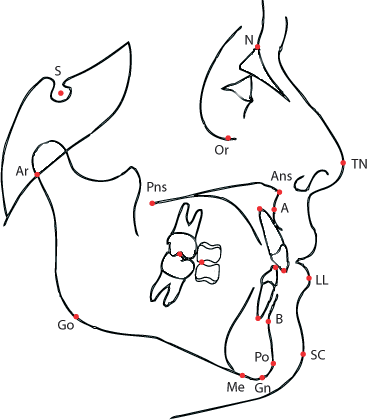
All the measurements are taken from x-ray scans using a set of reference points established using a map like the following:
> load("prepd-ortho.rda")
> str(ortho)
'data.frame':	143 obs. of  17 variables:
 $ ID       : Factor w/ 143 levels "P001","P002",..: 1 2 4 5 6 7 9 10 11 13 ...
 $ Treatment: Factor w/ 3 levels "NT","TB","TG": 1 1 1 1 1 1 1 1 3 1 ...
 $ Growth   : Factor w/ 2 levels "Bad","Good": 1 2 1 1 1 2 2 2 1 1 ...
 $ ANB      : num  -5.2 -1.7 -3.1 -1.3 0.4 1.5 -0.1 0.5 0.2 0.2 ...
 $ IMPA     : num  75.9 77.2 89.8 98.7 90.5 96.9 85.9 92 91.7 82.2 ...
 $ PPPM     : num  30.2 27 19.8 21.5 26.5 25.2 21.2 19.5 31.1 22.7 ...
 $ CoA      : num  83.4 91.3 78.6 96.4 83.3 88 85 77.1 88.8 77.5 ...
 $ GoPg     : num  77.9 84.1 67.3 75.6 74.7 72.8 75.2 65.2 76.2 67.8 ...
 $ CoGo     : num  50.1 59.2 50.4 65.7 51.3 58 54.9 44.8 53.3 44.5 ...
 $ ANB2     : num  -8.4 -2.3 -4.7 -2.4 -0.7 0.9 -1.3 0.4 0.8 -2.8 ...
 $ IMPA2    : num  71.7 81 83.8 86.6 83.8 95.8 87.7 93.6 92.3 82.6 ...
 $ PPPM2    : num  29.1 26.5 16.7 19.4 26.5 24.3 19.4 17.2 30.2 20.1 ...
 $ CoA2     : num  84.4 93.9 82.9 110.5 91 ...
 $ GoPg2    : num  81.9 84 71.5 96.3 83.5 71.8 76.9 69.3 81.3 82.5 ...
 $ CoGo2    : num  53.8 60.6 57.5 83.2 62.3 58.9 57.9 44.9 62 61 ...
 $ T1       : num  12 13 9 7 9 14 10 7 11 6 ...
 $ T2       : num  17 16 14 16 14 17 13 9 14 17 ...
Preprocessing and exploratory data analysis
Firstly, we create a data frame with the differences for all the variables and with Growth
and Treatment.
> diff = data.frame(
+           dANB = ortho$ANB2 - ortho$ANB,
+           dPPPM = ortho$PPPM2 - ortho$PPPM,
+           dIMPA = ortho$IMPA2 - ortho$IMPA,
+           dCoA = ortho$CoA2 - ortho$CoA,
+           dGoPg = ortho$GoPg2 - ortho$GoPg,
+           dCoGo = ortho$CoGo2 - ortho$CoGo,
+           dT = ortho$T2 - ortho$T1,
+           Growth = as.numeric(ortho$Growth) - 1,
+           Treatment = as.numeric(ortho$Treatment != "NT")
+ )
The Growth and Treatment variables carry redundant information on the
prognosis of the patient, as evidenced by the difference in the proportions of patients with good
Growth between TB and TG.
> table(ortho[, c("Treatment", "Growth")])
         Growth
Treatment Bad Good
       NT  51   26
       TB  10    3
       TG  24   29
To avoid the confounding that would result from including both variables in the model we re-code
Treatment as a binary variable for which 0 means NT and
1 means either TB or TG. Similarly, we re-code Growth
with 0 meaning Bad and 1 meaning Good.
> table(diff[, c("Treatment", "Growth")])
         Growth
Treatment  0  1
        0 51 26
        1 34 32
Since we will be using Gaussian BNs for the analysis, it also interesting to check whether the variables are normally distributed, at least marginally; and from the plots below that does not seem to be the case for all of them.
> par(mfrow = c(2, 3), mar = c(4, 2, 2, 2))
> for (var in c("dANB", "dPPPM", "dIMPA", "dCoA", "dGoPg", "dCoGo")) {

+   x = diff[, var]
+   hist(x, prob = TRUE, xlab = var, ylab = "", main = "", col = "ivory")
+   lines(density(x), lwd = 2, col = "tomato")
+   curve(dnorm(x, mean = mean(x), sd = sd(x)), from = min(x), to = max(x),
+     add = TRUE, lwd = 2, col = "steelblue")

+ }

Are the variables linked by linear relationships? Some of them are, but not all.
> pairs(diff[, setdiff(names(diff), c("Growth", "Treatment"))],
+   upper.panel = function(x, y, ...) {
+     points(x = x, y = y, col = "grey")
+     abline(coef(lm(y ~ x)), col = "tomato", lwd = 2)
+   },
+   lower.panel = function(x, y, ...) {
+     par(usr = c(0, 1, 0, 1))
+     text(x = 0.5, y = 0.5, round(cor(x, y), 2), cex = 2)
+   }
+ )

Finally, we can take a look at whether the variables cluster in any ways since variables that cluster together are more likely to be linked in the BN.
> library(gplots)
> diff.delta = sapply(diff[, 1:6], function(x) x / diff$dT)
> rho = cor(data.frame(diff.delta, Growth = diff$Growth, Treatment = diff$Treatment))
> palette.breaks = seq(0, 1, 0.1)
> par(oma = c(2, 2, 2, 1))
> heatmap.2(rho, scale = "none", trace = "none", revC = TRUE, breaks = palette.breaks)

We can see to clusters in the heatmap: the first comprises dCoGo, dGoPg
and dCoA and the second comprises Treatment, dANB and
dCoA. The first cluster is clinically interesting because it includes
Treatment and two variables that are both related to Down's point A, which gives some
clues about where the main effect of the treatment is.
> ug = empty.graph(colnames(rho))
> amat(ug) = (rho > 0.4) + 0L - diag(1L, nrow(rho))
> graphviz.plot(ug, layout = "fdp", shape = "ellipse")

Model #1: a static Bayesian network as a difference model
Here we will try to model the data using the differences we save in diff instead of
the raw values; and we will use a GBN treating since all variables are numeric. Modelling
differences leads to local distributions that are regression models of the form

where  and so
forth for the other regressors. We can rewrite such regression as
and so
forth for the other regressors. We can rewrite such regression as

which is a set of differential equations that models the rates of change whose relationships are assumed to be well approximated by linear relationships. This formulation, however, still implies that the raw values change linearly over time, because the rate of change depends on the rates of change of other variables but not on time itself. To have a nonlinear trend we would need

Furthermore, including the Growth variable means that we can have
regression models of the form

thus allowing for different rates of change depending on whether the patient shows positive developments or not in the malocclusion and whether he is being treated or not.
Learning the Bayesian network
Learning the structure
The first step in learning a BN is learning its structure, that is, the DAG
. We can do that using data (from the diff data frame)
combined with prior knowledge; incorporating the latter reduces the space of the models we will have to explore and
leads to more robust BNs. A straightforward way of doing that is to blacklist arcs that encode relationships we
know not be possible/real (we do not want them in , even if noisy data
might suggest they are real); and to whitelist arcs that encode relationship we know to exist (we do want them
in , even if they are not apparent from the data).
A blacklist is just a matrix (or a data frame) with a from and a to
columns that lists the arcs we do not want in the BN.
- We blacklist any arc pointing to
dT,TreatmentandGrowthfrom the orthodontic variables. - We blacklist the arc from
dTtoTreatment. This means that whether a patient is treated does not change over time. - We blacklist the arc from
GrowthtodTandTreatment. This means that whether a patient is treated does not change over time, and it obviously does not change depending on the prognosis.
> bl = tiers2blacklist(list("dT", "Treatment", "Growth",
+        c("dANB", "dPPPM", "dIMPA", "dCoA", "dGoPg", "dCoGo")))
> bl = rbind(bl, c("dT", "Treatment"), c("Treatment", "dT"))
> bl
      from        to
 [1,] "Treatment" "dT"
 [2,] "Growth"    "dT"
 [3,] "dANB"      "dT"
 [4,] "dPPPM"     "dT"
 [5,] "dIMPA"     "dT"
 [6,] "dCoA"      "dT"
 [7,] "dGoPg"     "dT"
 [8,] "dCoGo"     "dT"
 [9,] "Growth"    "Treatment"
[10,] "dANB"      "Treatment"
[11,] "dPPPM"     "Treatment"
[12,] "dIMPA"     "Treatment"
[13,] "dCoA"      "Treatment"
[14,] "dGoPg"     "Treatment"
[15,] "dCoGo"     "Treatment"
[16,] "dANB"      "Growth"
[17,] "dPPPM"     "Growth"
[18,] "dIMPA"     "Growth"
[19,] "dCoA"      "Growth"
[20,] "dGoPg"     "Growth"
[21,] "dCoGo"     "Growth"
[22,] "dT"        "Treatment"
[23,] "Treatment" "dT"
A whitelist has the same structure as a blacklist.
- We whitelist the dependence structure
dANB→dIMPA←dPPPM. - We whitelist the arc from
dTtoGrowthwhich allows the prognosis to change over time.
> wl = matrix(c("dANB", "dIMPA",
+               "dPPPM", "dIMPA",
+               "dT", "Growth"),
+         ncol = 2, byrow = TRUE, dimnames = list(NULL, c("from", "to")))
> wl
     from    to
[1,] "dANB"  "dIMPA"
[2,] "dPPPM" "dIMPA"
[3,] "dT"    "Growth"
A simple approach to learn would be to find the network structure
with the best goodness-of-fit on the whole data. For instance, using hc() with the default score
(BIC) and the whole diff data frame:
> dag = hc(diff, whitelist = wl, blacklist = bl)
> dag
  Bayesian network learned via Score-based methods

  model:
   [dT][Treatment][Growth|dT:Treatment][dANB|Growth:Treatment]
   [dCoA|dANB:dT:Treatment][dGoPg|dANB:dCoA:dT:Growth]
   [dCoGo|dANB:dCoA:dT:Growth][dPPPM|dCoGo][dIMPA|dANB:dPPPM:Treatment]
  nodes:                                 9
  arcs:                                  19
    undirected arcs:                     0
    directed arcs:                       19
  average markov blanket size:           5.33
  average neighbourhood size:            4.22
  average branching factor:              2.11

  learning algorithm:                    Hill-Climbing
  score:                                 BIC (Gauss.)
  penalization coefficient:              2.481422
  tests used in the learning procedure:  157
  optimized:                             TRUE
To check how hc() actually built the network, and how various arcs were (not) included in
, we can just run the command above again with
debug = TRUE:
----------------------------------------------------------------
* starting from the following network:

  Random/Generated Bayesian network

  model:
   [dANB][dPPPM][dCoA][dGoPg][dCoGo][dT][Treatment][dIMPA|dANB:dPPPM]
   [Growth|dT]
  nodes:                                 9
  arcs:                                  3
    undirected arcs:                     0
    directed arcs:                       3
  average markov blanket size:           0.89
  average neighbourhood size:            0.67
  average branching factor:              0.33

  generation algorithm:                  Empty

* current score: -2938.765
* whitelisted arcs are:
     from    to
[1,] "dANB"  "dIMPA"
[2,] "dPPPM" "dIMPA"
[3,] "dT"    "Growth"
* blacklisted arcs are:
      from        to
 [1,] "Treatment" "dT"
 [2,] "Growth"    "dT"
 [3,] "dANB"      "dT"
 [4,] "dPPPM"     "dT"
 [5,] "dIMPA"     "dT"
 [6,] "dCoA"      "dT"
 [7,] "dGoPg"     "dT"
 [8,] "dCoGo"     "dT"
 [9,] "Growth"    "Treatment"
[10,] "dANB"      "Treatment"
[11,] "dPPPM"     "Treatment"
[12,] "dIMPA"     "Treatment"
[13,] "dCoA"      "Treatment"
[14,] "dGoPg"     "Treatment"
[15,] "dCoGo"     "Treatment"
[16,] "dANB"      "Growth"
[17,] "dPPPM"     "Growth"
[18,] "dIMPA"     "Growth"
[19,] "dCoA"      "Growth"
[20,] "dGoPg"     "Growth"
[21,] "dCoGo"     "Growth"
[22,] "dT"        "Treatment"
[23,] "dIMPA"     "dANB"
[24,] "dIMPA"     "dPPPM"
* caching score delta for arc dANB -> dPPPM (-1.539098).
* caching score delta for arc dANB -> dIMPA (0.856161).
* caching score delta for arc dANB -> dCoA (8.901223).
* caching score delta for arc dANB -> dGoPg (-0.934598).
* caching score delta for arc dANB -> dCoGo (-2.120463).
* caching score delta for arc dPPPM -> dIMPA (-2.846313).
* caching score delta for arc dPPPM -> dCoA (4.291717).
* caching score delta for arc dPPPM -> dGoPg (1.305411).
* caching score delta for arc dPPPM -> dCoGo (9.452469).
* caching score delta for arc dIMPA -> dCoA (-2.435017).
* caching score delta for arc dIMPA -> dGoPg (-2.106127).
* caching score delta for arc dIMPA -> dCoGo (-2.486190).
* caching score delta for arc dCoA -> dIMPA (-1.192979).
* caching score delta for arc dCoA -> dGoPg (93.911397).
* caching score delta for arc dCoA -> dCoGo (68.650076).
* caching score delta for arc dGoPg -> dIMPA (-0.413628).
* caching score delta for arc dGoPg -> dCoGo (56.572414).
* caching score delta for arc dCoGo -> dIMPA (-1.167656).
* caching score delta for arc dT -> dANB (-1.527379).
* caching score delta for arc dT -> dPPPM (0.063080).
* caching score delta for arc dT -> dIMPA (-0.659672).
* caching score delta for arc dT -> dCoA (51.008025).
* caching score delta for arc dT -> dGoPg (76.176115).
* caching score delta for arc dT -> dCoGo (51.756230).
* caching score delta for arc dT -> Growth (1.912126).
* caching score delta for arc Growth -> dANB (9.490576).
* caching score delta for arc Growth -> dPPPM (-2.486674).
* caching score delta for arc Growth -> dIMPA (-0.332326).
* caching score delta for arc Growth -> dCoA (-2.437912).
* caching score delta for arc Growth -> dGoPg (0.391115).
* caching score delta for arc Growth -> dCoGo (2.469922).
* caching score delta for arc Treatment -> dANB (23.927293).
* caching score delta for arc Treatment -> dPPPM (-1.158971).
* caching score delta for arc Treatment -> dIMPA (1.593137).
* caching score delta for arc Treatment -> dCoA (28.348451).
* caching score delta for arc Treatment -> dGoPg (11.934805).
* caching score delta for arc Treatment -> dCoGo (11.530382).
* caching score delta for arc Treatment -> Growth (0.358153).
----------------------------------------------------------------
* trying to add one of 45 arcs.
  > trying to add dANB -> dPPPM.
    > delta between scores for nodes dANB dPPPM is -1.539098.
  > trying to add dANB -> dCoA.
    > delta between scores for nodes dANB dCoA is 8.901223.
    @ adding dANB -> dCoA.
  > trying to add dANB -> dGoPg.
    > delta between scores for nodes dANB dGoPg is -0.934598.
  > trying to add dANB -> dCoGo.
    > delta between scores for nodes dANB dCoGo is -2.120463.
  > trying to add dPPPM -> dANB.
...
As for plotting , the key function is graphviz.plot()
which provides a simple interface to the Rgraphviz package.
> graphviz.plot(dag, shape = "ellipse", highlight = list(arcs = wl))

However, the quality of dag crucially depends on whether variables are normally
distributed and on whether the relationships that link them are linear; from the exploratory
analysis it is not clear that is the case for all of them. We also have no idea about which arcs
represent strong relationships, meaning that they are resistant to perturbations of the data. We
can address both issues using boot.strength() to:
- resample the data using bootstrap;
- learn a separate network from each bootstrap sample;
- check how often each possible arc appears in the networks;
- construct a consensus network with the arcs that appear more often.
> str.diff = boot.strength(diff, R = 200, algorithm = "hc",
+             algorithm.args = list(whitelist = wl, blacklist = bl))
> head(str.diff)
  from    to strength direction
1 dANB dPPPM    0.590 0.3771186
2 dANB dIMPA    1.000 1.0000000
3 dANB  dCoA    0.820 0.6615854
4 dANB dGoPg    0.445 0.7191011
5 dANB dCoGo    0.610 0.8278689
6 dANB    dT    0.145 0.0000000
The return value of boot.strength() includes, for each pair of nodes, the
strength of the arc that connects them (say, how often we observe dANB
→ dPPPM or dPPPM → dANB) and the strength of its
direction (say, how often we observe dANB → dPPPM
when we observe an arc at all between dANB and dPPPM).
boot.strength() also computes the threshold that will be used to decide whether an
arc is strong enough to be included in the consensus network.
> attr(str.diff, "threshold")
[1] 0.585
So, averaged.network() takes all the arcs with a strength of at least
0.585 and returns an averaged consensus network, unless a
different threshold is specified.
> avg.diff = averaged.network(str.diff)
Plotting avg.diff with Rgraphviz, we can incorporate the information
we now have on the strength of the arcs by using strength.plot() instead of
graphviz.plot(). strength.plot() takes the same arguments as
graphviz.plot() plus a threshold and a set of cutpoints to
determine how to format each arc depending on its strength.
> strength.plot(avg.diff, str.diff, shape = "ellipse", highlight = list(arcs = wl))

How can we compare the averaged network (avg.diff) with the network we originally
learned in from all the data (dag)? The most qualitative way is to plot the two networks
side by side, with the nodes in the same positions, and highlight the arcs that appear in one network
and not in the other, or that appear with different directions.
> par(mfrow = c(1, 2))
> graphviz.compare(avg.diff, dag, shape = "ellipse", main = c("averaged DAG", "single DAG"))

We can see that the arcs Treatment → dIMPa, dANB
→ dGoPg and dCoGo → dPPPM appear only in the averaged
network, and that dPPPM → dANB appears only in the network we learned
from all the data. We can assume that the former three arcs were hidden by the noisiness of the data
combined with the small sample sizes and departures from normality. The programmatic equivalent of
graphviz.compare() is simply called compare(): it can return the number of
true positives (arcs that appear in both networks) and false positives/negatives (arcs that appear in
only one of thew two networks),
> compare(avg.diff, dag)
$tp
[1] 16

$fp
[1] 3

$fn
[1] 1
or the arcs themselves, with arcs = TRUE.
> compare(avg.diff, dag, arcs = TRUE)
$tp
      from        to
 [1,] "dANB"      "dIMPA"
 [2,] "dANB"      "dCoA"
 [3,] "dANB"      "dCoGo"
 [4,] "dPPPM"     "dIMPA"
 [5,] "dCoA"      "dGoPg"
 [6,] "dCoA"      "dCoGo"
 [7,] "dT"        "dCoA"
 [8,] "dT"        "dGoPg"
 [9,] "dT"        "dCoGo"
[10,] "dT"        "Growth"
[11,] "Growth"    "dANB"
[12,] "Growth"    "dGoPg"
[13,] "Growth"    "dCoGo"
[14,] "Treatment" "dANB"
[15,] "Treatment" "dIMPA"
[16,] "Treatment" "dCoA"

$fp
     from        to
[1,] "dCoGo"     "dPPPM"
[2,] "Treatment" "Growth"
[3,] "dANB"      "dGoPg"

$fn
     from    to
[1,] "dPPPM" "dANB"
But are all the arc directions well established, in light of the fact that the networks are learned
with BIC which is score equivalent? Looking at the CPDAGs for dag and avg.diff
(and taking whitelists and blacklists into account), we see that there are no undirected arcs. All arcs
directions are uniquely identified.
> undirected.arcs(cpdag(dag, wlbl = TRUE))
from to
> avg.diff$learning$whitelist = wl
> avg.diff$learning$blacklist = bl
> undirected.arcs(cpdag(avg.diff, wlbl = TRUE))
from to
Finally we can combine the compare() and cpdag() to perform a principled
comparison in which we say two arcs are different if they have been uniquely identified being different.
> compare(cpdag(avg.diff, wlbl = TRUE), cpdag(dag, wlbl = TRUE))
$tp
[1] 16

$fp
[1] 3

$fn
[1] 1
It is also a good idea to look at the threshold with respect to the distribution of the arc strengths:
the averaged network is fairly dense (17 arcs for 9
nodes) and it is difficult to read.
> plot(str.diff)
> abline(v = 0.75, col = "tomato", lty = 2, lwd = 2)
> abline(v = 0.85, col = "steelblue", lty = 2, lwd = 2)

Hence it would be good to increase the threshold a bit and to drop a few more arcs. Looking at the plot above, two natural choices for a higher threshold are 0.75 (red dashed line) and 0.85 (blue dashed line) because of the gaps in the distribution of the arc strengths.
> nrow(str.diff[str.diff$strength > attr(str.diff, "threshold") &
+               str.diff$direction > 0.5, ])
[1] 18
> nrow(str.diff[str.diff$strength > 0.75 & str.diff$direction > 0.5, ])
[1] 15
> nrow(str.diff[str.diff$strength > 0.85 & str.diff$direction > 0.5, ])
[1] 12
The simpler network we obtain by setting threshold = 0.85 in averaged.network()
is shown below; it is certainly easier to reason with from a qualitative point of view.
> avg.simpler = averaged.network(str.diff, threshold = 0.85)
> strength.plot(avg.simpler, str.diff, shape = "ellipse", highlight = list(arcs = wl))

Learning the parameters
Having learned the structure, we can now learn the parameters. Since we are working with continuous variables, we choose to model them with a GBN. Hence if we fit the parameters of the network using their maximum likelihood estimate we have that each local distribution is a classic linear regression.
> fitted.simpler = bn.fit(avg.simpler, diff)
> fitted.simpler
  Bayesian network parameters

  Parameters of node dANB (Gaussian distribution)

Conditional density: dANB | Growth + Treatment
Coefficients:
(Intercept)       Growth    Treatment
  -1.560045     1.173979     1.855994
Standard deviation of the residuals: 1.416369

  Parameters of node dPPPM (Gaussian distribution)

Conditional density: dPPPM | dCoGo
Coefficients:
(Intercept)        dCoGo
  0.1852132   -0.2317049
Standard deviation of the residuals: 2.50641

  Parameters of node dIMPA (Gaussian distribution)

Conditional density: dIMPA | dANB + dPPPM
Coefficients:
(Intercept)         dANB        dPPPM
 -1.3826102    0.4074842   -0.5018133
Standard deviation of the residuals: 4.896511

  Parameters of node dCoA (Gaussian distribution)

Conditional density: dCoA | Treatment
Coefficients:
(Intercept)    Treatment
   3.546753     5.288095
Standard deviation of the residuals: 3.615473

  Parameters of node dGoPg (Gaussian distribution)

Conditional density: dGoPg | dCoA + dT
Coefficients:
(Intercept)         dCoA           dT
 -0.6088760    0.6998461    0.8816657
Standard deviation of the residuals: 2.373902

  Parameters of node dCoGo (Gaussian distribution)

Conditional density: dCoGo | dCoA + dT + Growth
Coefficients:
(Intercept)         dCoA           dT       Growth
  1.5378012    0.5932982    0.5240202   -2.0302255
Standard deviation of the residuals: 2.428629

  Parameters of node dT (Gaussian distribution)

Conditional density: dT
Coefficients:
(Intercept)
   4.706294
Standard deviation of the residuals: 2.550427

  Parameters of node Growth (Gaussian distribution)

Conditional density: Growth | dT
Coefficients:
(Intercept)           dT
 0.48694013  -0.01728446
Standard deviation of the residuals: 0.4924939

  Parameters of node Treatment (Gaussian distribution)

Conditional density: Treatment
Coefficients:
(Intercept)
  0.4615385
Standard deviation of the residuals: 0.5002708
We can easily confirm that is the case by comparing the models produced by bn.fit() and
lm(), for instance dANB.
> fitted.simpler$dANB
  Parameters of node dANB (Gaussian distribution)

Conditional density: dANB | Growth + Treatment
Coefficients:
(Intercept)       Growth    Treatment
  -1.560045     1.173979     1.855994
Standard deviation of the residuals: 1.416369
> summary(lm(dANB ~ Growth + Treatment, data = diff))
Call:
lm(formula = dANB ~ Growth + Treatment, data = diff)

Residuals:
    Min      1Q  Median      3Q     Max
-3.5400 -0.8139 -0.0959  0.7861  5.2861

Coefficients:
            Estimate Std. Error t value Pr(>|t|)
(Intercept)  -1.5600     0.1812  -8.609 1.37e-14 ***
Growth        1.1740     0.2440   4.812 3.82e-06 ***
Treatment     1.8560     0.2403   7.724 1.96e-12 ***
---
Signif. codes:  0 '***' 0.001 '**' 0.01 '*' 0.05 '.' 0.1 ' ' 1

Residual standard error: 1.416 on 140 degrees of freedom
Multiple R-squared:  0.407,	Adjusted R-squared:  0.3985
F-statistic: 48.04 on 2 and 140 DF,  p-value: < 2.2e-16
Can we have problems with collinearity? In theory it is possible, but it is mostly not an issue in practice with
network structures learning from data. The reason is that if two variables
 and
and  are collinear,
after adding (say) ←
then ←
will no longer significantly improve BIC because
and provide (to
some extent) the same information on .
are collinear,
after adding (say) ←
then ←
will no longer significantly improve BIC because
and provide (to
some extent) the same information on .
> library(MASS)
>
> # a three-dimensional multivariate Gaussian.
> mu = rep(0, 3)
> R = matrix(c(1,   0.6, 0.5,
+              0.6, 1,   0,
+              0.5, 0,   1),
+       ncol = 3, dimnames = list(c("y", "x1", "x2"), c("y", "x1", "x2")))
>
> # gradually increase the correlation between the explanatory variables.
> for (rho in seq(from = 0, to = 0.85, by = 0.05)) {

+   # update the correlation matrix and generate the data.
+   R[2, 3] = R[3, 2] = rho
+   data = as.data.frame(mvrnorm(10000, mu, R))
+   # compare the linear models (full vs reduced).
+   cat("rho:", sprintf("%.2f", rho), "difference in BIC:",
+     - 2 * (BIC(lm(y ~ x1 + x2, data = data)) - BIC(lm(y ~ x1, data = data))), "\n")

+ }#FOR
rho: 0.00 difference in BIC: 9578.292
rho: 0.05 difference in BIC: 8514.269
rho: 0.10 difference in BIC: 7240.748
rho: 0.15 difference in BIC: 6208.321
rho: 0.20 difference in BIC: 5162.806
rho: 0.25 difference in BIC: 4918.283
rho: 0.30 difference in BIC: 3842.159
rho: 0.35 difference in BIC: 3209.251
rho: 0.40 difference in BIC: 2541.455
rho: 0.45 difference in BIC: 2133.278
rho: 0.50 difference in BIC: 1780.175
rho: 0.55 difference in BIC: 1215.249
rho: 0.60 difference in BIC: 963.8037
rho: 0.65 difference in BIC: 687.7402
rho: 0.70 difference in BIC: 322.9057
rho: 0.75 difference in BIC: 165.8649
rho: 0.80 difference in BIC: 7.844978
rho: 0.85 difference in BIC: -17.28751
If parameter estimates are problematic for any reason, we can replace them with a new set of estimates from a different approach.
> fitted.new = fitted.simpler
> fitted.new$dANB = list(coef = c(-1, 2, 2), sd = 1.5)
> fitted.new$dANB
  Parameters of node dANB (Gaussian distribution)

Conditional density: dANB | Growth + Treatment
Coefficients:
(Intercept)       Growth    Treatment
         -1            2            2
Standard deviation of the residuals: 1.5
> fitted.new$dANB = penalized(diff$dANB, penalized = diff[, parents(avg.simpler, "dANB")],
+                     lambda2 = 20, model = "linear", trace = FALSE)
> fitted.new$dANB
  Parameters of node dANB (Gaussian distribution)

Conditional density: dANB | Growth + Treatment
Coefficients:
(Intercept)       Growth    Treatment
 -1.1175168    0.8037963    1.2224956
Standard deviation of the residuals: 1.469436
Model validation
There are two main approaches to validate a BN.
- Looking just at the network structure: if the main goal of learning the BN is to identify arcs and pathways, which is often the case when the BN is interpreted as a causal model, we can perform what is essentially a path analysis and studying arc strengths.
- Looking at the BN as a whole, including the parameters: if the main goal of learning
the BN is to use it as an expert model, then we may like to:
- predict the values of one or more variables for new individuals, based on the values of some other variables; and
- comparing the results of CP queries to expert knowledge to confirm the BN reflects the best knowledge available on the phenomenon we are modelling.
Predictive accuracy
We can measure predictive accuracy of our chosen learning strategy in the usual way, with
cross-validation. bnlearn provides the bn.cv() function for this task,
which implements:
- k-fold cross-validation;
- cross-validation with user-specified folds;
- hold-out cross-validation
for:
- structure learning algorithms (the structure and the parameters are learned from data);
- parameter learning algorithms (the structure is provided by the user, the parameters are learned from the data).
The return value of bn.cv() is an object of class bn.kcv (or
bn.kcv-list for multiple cross-validation runs, see ?"bn.kcv class") that
contains:
- the row indexes for the observations used as the test set;
- a
bn.fitobject learned from the training data; - the value of the loss function;
- fitted and predicted values for loss functions that require them.
First we check Growth, which encodes the evolution of malocclusion (0
meaning Bad and 1 meaning Good). We check it transforming it
back into discrete variable and computing the prediction error.
> xval = bn.cv(diff, bn = "hc", algorithm.args = list(blacklist = bl, whitelist = wl),
+   loss = "cor-lw", loss.args = list(target = "Growth", n = 200), runs = 10)
>
> err = numeric(10)
>
> for (i in 1:10) {

+   tt = table(unlist(sapply(xval[[i]], '[[', "observed")),
+              unlist(sapply(xval[[i]], '[[', "predicted")) > 0.50)

+   err[i] = (sum(tt) - sum(diag(tt))) / sum(tt)

+ }#FOR
>
> summary(err)
   Min. 1st Qu.  Median    Mean 3rd Qu.    Max.
 0.2587  0.2727  0.2867  0.2839  0.2937  0.3077
The other variables are continuous, so we can estimate their predictive correlation instead.
> predcor = structure(numeric(6),
+             names = c("dCoGo", "dGoPg", "dIMPA", "dCoA", "dPPPM", "dANB"))
>
> for (var in names(predcor)) {

+   xval = bn.cv(diff, bn = "hc", algorithm.args = list(blacklist = bl, whitelist = wl),
+            loss = "cor-lw", loss.args = list(target = var, n = 200), runs = 10)

+     predcor[var] = mean(sapply(xval, function(x) attr(x, "mean")))

+ }#FOR
>
> round(predcor, digits = 3)
dCoGo dGoPg dIMPA  dCoA dPPPM  dANB
0.849 0.904 0.220 0.922 0.413 0.658
> mean(predcor)
[1] 0.6609281
In both cases we use the *-lw variants of the loss functions, which perform prediction
using posterior expected values computed from all the other variables. The base loss functions
(cor, mse, pred) predict the values of each node just from their
parents, which is not meaningful when working on nodes with few or no parents.
Confirming with expert knowledge
The other way to confirm whether the BN makes sense is to treat it as a working model of the world and to see whether it expresses key facts about the world that were not used as prior knowledge during learning. (Otherwise we would just be getting back the information we put in the prior!) Some examples:
- "An excessive growth of
CoGoshould induce a reduction inPPPM."
We test this hypothesis by generating samples for the BN stored infitted.simplerfor bothdCoGoanddPPPMand assuming no treatment is taking place. AsdCoGoincreases (which indicates an increasingly rapid growth)dPPPMbecomes increasingly negative (which indicates a reduction in the angle assuming the angle is originally positive.> sim = cpdist(fitted.simpler, nodes = c("dCoGo", "dPPPM"), n = 10^4, + evidence = (Treatment < 0.5)) > plot(sim, col = "grey") > abline(v = 0, col = 2, lty = 2, lwd = 2) > abline(h = 0, col = 2, lty = 2, lwd = 2) > abline(coef(lm(dPPPM ~ dCoGo, data = sim)), lwd = 2)

- "A small growth of
CoGoshould induce an increase inPPPM."
From the figure above, a negative or null growth of CoGo (dCoGo⋜ 0) corresponds to a positive growth in PPPM with probability ≈ 0.60. For a small growth of CoGo (dCoGo∈ [0, 2]) unfortunatelydPPPM⋜ 0 with probability ≈ 0.50 so the BN does not support this hypothesis.> nrow(sim[(sim$dCoGo <= 0) & (sim$dPPPM > 0), ]) / nrow(sim[(sim$dCoGo <= 0), ])
[1] 0.6112532
> nrow(sim[(sim$dCoGo > 0) & (sim$dCoGo < 2) & (sim$dPPPM > 0), ]) /
+   nrow(sim[(sim$dCoGo) > 0 & (sim$dCoGo < 2),  ])
[1] 0.4781784
- "If
ANBdecreases,IMPAdecreases to compensate."
Testing by simulation as before, we are looking for negative values ofdANB(which indicate a decrease assuming the angle is originally positive) associated with negative values ofIMPA(same). From the figure belowdANBis proportional todIMPA, so a decrease in one suggests a decrease in the other; the mean trend (the black line) is negative for both at the same time.> sim = cpdist(fitted.simpler, nodes = c("dIMPA", "dANB"), n = 10^4, + evidence = (Treatment < 0.5)) > plot(sim, col = "grey") > abline(v = 0, col = 2, lty = 2, lwd = 2) > abline(h = 0, col = 2, lty = 2, lwd = 2) > abline(coef(lm(dIMPA ~ dANB, data = sim)), lwd = 2)

- "If
GoPgincreases strongly, then bothANBandIMPAdecrease." If we simulatedGoPg,dANBanddIMPAfrom the BN assumingdGoPg> 5 (i.e.GoPgis increasing) we estimate the probability thatdANB> 0 (i.e.ANBis increasing) at ≈ 0.70 and thatdIMPA< 0 at only ≈ 0.58.> sim = cpdist(fitted.simpler, nodes = c("dGoPg", "dANB", "dIMPA"), n = 10^4, + evidence = (dGoPg > 5) & (Treatment < 0.5)) > nrow(sim[(sim$dGoPg > 5) & (sim$dANB < 0), ]) / nrow(sim[(sim$dGoPg > 5), ])
[1] 0.6954162
> nrow(sim[(sim$dGoPg > 5) & (sim$dIMPA < 0), ]) / nrow(sim[(sim$dGoPg > 5), ])
[1] 0.5756936
- "Therapy attempts to stop the decrease of
ANB. If we fixANBis there any difference treated and untreated patients?"
First, we can check the relationship between treatment and growth for patients that havedANB≈ 0 without any intervention (i.e. using the BN we learned from the data).The estimated P(> sim = cpdist(fitted.simpler, nodes = c("Treatment", "Growth"), n = 5 * 10^4, + evidence = abs(dANB) < 0.1) > tab = table(TREATMENT = sim$Treatment < 0.5, GOOD.GROWTH = sim$Growth > 0.5) > round(prop.table(tab, margin = 1), 2)
GOOD.GROWTH TREATMENT FALSE TRUE FALSE 0.61 0.39 TRUE 0.49 0.51GOOD.GROWTH∣TREATMENT) is different for treated and untreated patients (≈ 0.65 versus ≈ 0.52).
If we simulate a formal intervention (a la Judea Pearl) and externally setdANB= 0 (thus making it independent from its parents and removing the corresponding arcs), we have thatGOOD.GROWTHhas practically the same distribution for both treated and untreated patients and thus becomes independent fromTREATMENT. This suggests that a favourable prognosis is indeed determined by preventing changes inANBand that other components of the treatment (if any) then become irrelevant.> avg.mutilated = mutilated(avg.simpler, evidence = list(dANB = 0)) > fitted.mutilated = bn.fit(avg.mutilated, diff) > fitted.mutilated$dANB = list(coef = c("(Intercept)" = 0), sd = 0) > sim = cpdist(fitted.mutilated, nodes = c("Treatment", "Growth"), n = 5 * 10^4, + evidence = TRUE) > tab = table(TREATMENT = sim$Treatment < 0.5, GOOD.GROWTH = sim$Growth > 0.5) > round(prop.table(tab, margin = 1), 2)
GOOD.GROWTH TREATMENT FALSE TRUE FALSE 0.57 0.43 TRUE 0.58 0.42 - "Therapy attempts to stop the decrease of
ANB. If we fixANBis there any difference between treated and untreated patients?"
One way of assessing this is to check whether the angle between point A and point B (ANB) changes between treated and untreated patients while keepingGoPgfixed.Assuming> sim.GoPg = cpdist(fitted.simpler, nodes = c("Treatment", "dANB", "dGoPg"), + evidence = abs(dGoPg) < 0.1)
GoPgdoes not change, the angle between point A and point B increases for treated patients (strongly negative values denote horizontal imbalance, so a positive rate of changes indicate a reduction in imbalance) and decreases for untreated patients (imbalance slowly worsens over time).> sim.GoPg$Treatment = c("UNTREATED", "TREATED")[(sim.GoPg$Treatment > 0.5) + 1L] > mean(sim.GoPg[sim.GoPg$Treatment == "UNTREATED", "dANB"])
[1] -0.8147217
> mean(sim.GoPg[sim.GoPg$Treatment == "TREATED", "dANB"])
[1] -0.4561556
> boxplot(dANB ~ Treatment, data = sim.GoPg)

Model #2: a dynamic Bayesian network
This BN was not included in the paper because it does not work as well as model #1 for prediction, while being more complex. This is inherent to dynamic BNs, that is, BNs that model stochastic processes: each variable is associated to a different node in each time point being modelled. (Typically, we assume that the process is Markov of order one, so we have two time points in the BN: t and t - 1.) However, we explore it for the purpose of illustrating how such a BN can be learned and used in bnlearn.
The data we use for this model are the raw data we stored into ortho at the beginning of
the analysis. However, we choose to use Treatement instead of Growth as the
variable to express the fact that subjects may be undertaking medical treatment. The reason is that
Growth is a variable that measures the prognosis at the time of the second measurement, and
its value is unknown at the time of the first measurement; whereas Treatment is the same at
both times.
Learning the structure
First, we divide the variables in three groups: variables at time t2, variables at time t1 = t2 - 1, and variables that are time-independent because they take the same value at t1 and t1.
> const = "Treatment"
> t2.variables = grep("2$", names(ortho), value = TRUE)
> t2.variables
[1] "ANB2" "IMPA2" "PPPM2" "CoA2" "GoPg2" "CoGo2" "T2"
> t1.variables = setdiff(names(ortho), c(t2.variables, const))
> t1.variables
[1] "ID" "ANB" "IMPA" "PPPM" "CoA" "GoPg" "CoGo" "T1"
Then we introduce a blacklist in which:
- We blacklist all arcs from the clinical variables to
T1,T2andTreatmentbecause we know that the age and the treatment regime are not dictated by the clinical measurements. - We blacklist all the arcs going into
Treatmentand into all the variables at time t1, because we assume that the arcs between the variables at time t1 are the same as the corresponding variables in time t2 and it's pointless to learn them twice. - We blacklist all the arcs from t2 to t1.
> roots = expand.grid(from = setdiff(names(ortho), c("T1", "T2", "Treatment")),
+                     to = c("T1", "T2", "Treatment"), stringsAsFactors = FALSE)
> empty.t1 = expand.grid(from = c(const, t1.variables), to = c(const, t1.variables),
+              stringsAsFactors = FALSE)
> bl = rbind(tiers2blacklist(list(t1.variables, t2.variables)), roots, empty.t1)
In contrast we only whitelist the arc T1 → T2, since the age at
the second measurement is obviously dependent on the age at the first.
> wl = data.frame(from = c("T1"), to = c("T2"))
Finally we can learn the structure of the BN with bl and wl.
> dyn.dag = tabu(ortho, blacklist = bl, whitelist = wl)
> dyn.dag
  Bayesian network learned via Score-based methods

  model:
   [ID][Treatment][ANB][IMPA][PPPM][CoA][GoPg][CoGo][T1]
   [ANB2|Treatment:ANB][T2|Treatment:T1][CoA2|Treatment:CoA:T1:T2]
   [CoGo2|ANB:CoA:CoGo:ANB2:CoA2:T2][PPPM2|PPPM:CoGo:CoGo2]
   [IMPA2|IMPA:ANB2:PPPM2][GoPg2|CoA:GoPg:ANB2:IMPA2:CoA2:T1:T2]
  nodes:                                 16
  arcs:                                  27
    undirected arcs:                     0
    directed arcs:                       27
  average markov blanket size:           7.38
  average neighbourhood size:            3.38
  average branching factor:              1.69

  learning algorithm:                    Tabu Search
  score:                                 BIC (cond. Gauss.)
  penalization coefficient:              2.481422
  tests used in the learning procedure:  800
  optimized:                             TRUE
It is clear that this BN is more complex than the previous one: it has more nodes
(16 vs 9), more arcs
(27 vs 19) and thus more parameters
(218 vs 37).
The best way of plotting this new model is to start with graphiz.plot() and to customise
it with more versatile commands from the Rgraphviz package. To this end we tell
graphviz.plot() not to plot anything since we are just interested in its return value.
> gR = graphviz.plot(dyn.dag, shape = "rectangle", render = FALSE)
Then we group variables (so that they are plotted close together) and we colour them to easily
distinguish const, t1.variables and t2.variables; and we
choose to draw the network from left to right instead of top to bottom.
> sg0 = list(graph = subGraph(const, gR), cluster = TRUE)
> sg1 = list(graph = subGraph(t1.variables, gR), cluster = TRUE)
> sg2 = list(graph = subGraph(t2.variables, gR), cluster = TRUE)
> gR = layoutGraph(gR, subGList = list(sg0, sg1, sg2),
+        attrs = list(graph = list(rankdir = "LR")))
> nodeRenderInfo(gR)$fill[t1.variables] = "tomato"
> nodeRenderInfo(gR)$fill[t2.variables] = "gold"
> renderGraph(gR)

As in the previous model, the treatment acts on ANB: the only arcs going out of
Treatment are Treatment → ANB2 and Treatment
→ CoA2. Again both child nodes are related to Down's point A.
Model averaging in structure learning
We would like to assess the stability of this dynamic BN structure much as we did for the static BN
earlier, and we can do that again with boot.strength() and averated.network().
> dyn.str = boot.strength(ortho, R = 200, algorithm = "tabu",
+             algorithm.args = list(blacklist = bl, whitelist = wl))
> plot(dyn.str)

> dyn.avg = averaged.network(dyn.str)
> dyn.avg
  Random/Generated Bayesian network

  model:
   [ID][Treatment][ANB][IMPA][PPPM][CoA][GoPg][CoGo][T1]
   [ANB2|Treatment:ANB][T2|Treatment:T1][CoA2|Treatment:CoA:T1:T2]
   [CoGo2|ANB:CoA:CoGo:ANB2:CoA2:T2][PPPM2|PPPM:ANB2:CoGo2]
   [IMPA2|IMPA:ANB2:PPPM2][GoPg2|CoA:GoPg:ANB2:IMPA2:CoA2:T1:T2]
  nodes:                                 16
  arcs:                                  27
    undirected arcs:                     0
    directed arcs:                       27
  average markov blanket size:           7.25
  average neighbourhood size:            3.38
  average branching factor:              1.69

  generation algorithm:                  Model Averaging
  significance threshold:                0.495
The averaged dyn.avg and dyn.dag are nearly identical: they differ by just
two arcs. This suggests that structure learning produces a stable output.
> unlist(compare(dyn.dag, dyn.avg))
tp fp fn
26  1  1
> par(mfrow = c(1, 2))
> graphviz.compare(dyn.dag, dyn.avg, shape = "rectangle")

Learning the parameters
Since Treatment is a discrete variable, the BN is a CLGBN. This means that continuous nodes
that have Treatment as a parent have a different parameterisation than the rest.
> dyn.fitted = bn.fit(dyn.avg, data = ortho)
> dyn.fitted$ANB2
  Parameters of node ANB2 (conditional Gaussian distribution)

Conditional density: ANB2 | Treatment + ANB
Coefficients:
                      0           1           2
(Intercept)  -1.2060815   0.0765252   1.0615742
ANB           0.9381008   0.3836207   0.8726937
Standard deviation of the residuals:
       0         1         2
1.548923  1.060644  1.460779
Discrete parents' configurations:
   Treatment
0         NT
1         TB
2         TG
As we can see, ANB2 depends on ANB (so, the same variable at the previous
time point) and Treatment. ANB is continuous, so it used as a regressor for
ANB2. Treatment is discrete, and determines the components of the mixture of
linear regressions.
Model validation and inference
We can ask another set of questions to this new model
- "How much does
ANBshift from the first to the second measurement with different treatment regimes?"
We can generate pairs of (ANB,ANB2) withcpdist()conditional onTreatmentbeing equal toNT,TBandTGand look at their distribution.We know that therapy attempts to stop the decrease of> nt = cpdist(dyn.fitted, nodes = c("ANB", "ANB2"), evidence = (Treatment == "NT")) > tb = cpdist(dyn.fitted, nodes = c("ANB", "ANB2"), evidence = (Treatment == "TB")) > tg = cpdist(dyn.fitted, nodes = c("ANB", "ANB2"), evidence = (Treatment == "TG")) > > effect = data.frame( + diff = c(nt[, 2] - nt[, 1], tb[, 2] - tb[, 1], tg[, 2] - tg[, 1]), + treatment = c(rep("NT", nrow(nt)), rep("TB", nrow(tb)), rep("TG", nrow(tg))) + ) > > by(effect$diff, effect$treatment, FUN = mean)
effect$treatment: NT
[1] -1.234719
--------------------------------------------------------
effect$treatment: TB
[1] 0.1322289
--------------------------------------------------------
effect$treatment: TG
[1] 1.135585
> col = c("steelblue", "gold", "tomato")
> lattice::densityplot(~ diff, groups = treatment, data = effect, col = col, lwd = 2, bw = 2, ylim = c(0, 0.20),
+   key = list(text = list(c("untreated", "treated with bad results", "treated with good results")),
+           col = col, lines = TRUE, corner = c(0.98, 0.98), lwd = 2))

ANB; and this is consistent with the fact that the distribution forNTis to the left of that forTBwhich is to the left ofTG. Untreated patient conditions continue to worsen; patients for which the treatment is not effective do not really improve but their conditions do not worsen either; and patients for which the treatment is effective improve. - "What does the evolution of
ANBlook like for different treatment regimes as the patient ages?"
Assuming an initial condition ofANBequal to 1 at age 5, we can iteratively predictANB2for the current age + 3 years to build a trajectory from childhood to adulthood. But this highlights one of the key limitations of this model: the assumption that probabilistic dependencies are linear means that the trajectory ofANB2will be approximately linear as well. That is unrealistic: we would stop the treatment before producing an imbalance in the other direction, and the growth process is bound to impact the skeletal growth in a non-linear way.In contrast, this is the simulated trajectory for an untreated patient with the same initial condition.> intervals = data.frame( + T1 = c(5, 8, 11, 14, 17), + T2 = c(8, 11, 14, 17, 20), + ANB = c(-1, NA, NA, NA, NA), + ANB2 = c(NA, NA, NA, NA, NA) + ) > > for (i in seq(nrow(intervals))) { + predictor = data.frame( + Treatment = factor("TG", levels = c("NT", "TB", "TG")), + T1 = intervals[i, "T1"], + T2 = intervals[i, "T2"], + ANB = intervals[i, "ANB"] + ) + intervals[i, "ANB2"] = predict(dyn.fitted, node = "ANB2", data = predictor, + method = "bayes-lw", from = names(predictor), n = 1000) + if (i < nrow(intervals)) + intervals[i + 1, "ANB"] = intervals[i, "ANB2"] + }#FOR > > print(intervals)
  T1 T2        ANB      ANB2
1  5  8 -1.0000000 0.2238031
2  8 11  0.2238031 1.2854308
3 11 14  1.2854308 2.2594550
4 14 17  2.2594550 3.0252664
5 17 20  3.0252664 3.7286357
The simulated trajectory forT1 T2 ANB ANB2 1 5 8 -1.000000 -2.165287 2 8 11 -2.165287 -3.209798 3 11 14 -3.209798 -4.230036 4 14 17 -4.230036 -5.085069 5 17 20 -5.085069 -5.940854
CoAis more realistic: it slows down with age. This is unlikeANB, and it happens becauseCoA2depends on bothT1andT2. (ANB2depends on neither.)> intervals = data.frame( + T1 = c(5, 8, 11, 14, 17), + T2 = c(8, 11, 14, 17, 20), + ANB = c(-1, NA, NA, NA, NA), + ANB2 = c(NA, NA, NA, NA, NA), + CoA = c(75, NA, NA, NA, NA), + CoA2 = c(NA, NA, NA, NA, NA) + ) > > for (i in seq(nrow(intervals))) { + predictor = data.frame( + Treatment = factor("TG", levels = c("NT", "TB", "TG")), + T1 = intervals[i, "T1"], + T2 = intervals[i, "T2"], + ANB = intervals[i, "ANB"], + CoA = intervals[i, "CoA"] + ) + # to perform a joint prediction, not currently possible with predict(). + dist = cpdist(dyn.fitted, nodes = c("ANB2", "CoA2"), + evidence = as.list(predictor), method = "lw") + weights = attr(dist, "weights") + intervals[i, "ANB2"] = weighted.mean(dist$ANB2, weights) + intervals[i, "CoA2"] = weighted.mean(dist$CoA2, weights) + if (i < nrow(intervals)) { + intervals[i + 1, "ANB"] = intervals[i, "ANB2"] + intervals[i + 1, "CoA"] = intervals[i, "CoA2"] + }#THEN + }#FOR > > print(intervals)
  T1 T2        ANB      ANB2       CoA      CoA2
1  5  8 -1.0000000 0.2005891  75.00000  85.95076
2  8 11  0.2005891 1.2635846  85.95076  93.59565
3 11 14  1.2635846 2.1510237  93.59565  98.49400
4 14 17  2.1510237 2.9463561  98.49400 100.97966
5 17 20  2.9463561 3.6514065 100.97966 101.41030
Tue Jul 16 12:28:11 2019 with bnlearn
4.5-20190701
and R version 3.0.2 (2013-09-25).

